Verification with the numbers beside it
Exact outputs, baseline comparisons, saturation checks and uncertainty intervals, with empirical and independent-review limits kept explicit.
What these checks establish
These are publisher-run numerical checks and synthetic controls. They test implementation, not physical truth. The measured memristor intake remains unfit, the elastomer experiment is unregistered, and no independent human replication has been logged.
Manufactured trajectories, including m = 0.95
q*(t) = sin(t), p*(t) = cos(t), 0 ≤ t ≤ 2
Interior: m*(t) = 0.4 + 0.1sin(0.7t)
Near upper boundary: m*(t) = 0.9 + 0.05sin(πt/2)
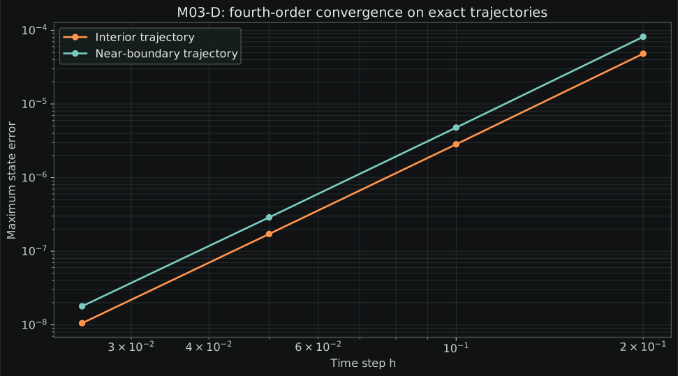
A known source vector is added to all three state equations. The near-boundary trajectory reaches 0.95 at t = 1. Maximum error is taken over q, p, m and all grid times. This checks integration order for the forced exact problem; the separate scalar test below exercises unmodified saturation dynamics.
| Writing / damping | Interior error, h=0.025 | Interior order | Near-boundary error, h=0.025 | Near-boundary order |
|---|---|---|---|---|
| drive / ratio | 1.044090e-08 | 3.9818 | 1.762501e-08 | 3.9900 |
| drive / coefficient | 1.039681e-08 | 4.0246 | 1.789562e-08 | 4.0058 |
| strain / ratio | 1.052900e-08 | 4.0041 | 1.765433e-08 | 3.9899 |
| strain / coefficient | 1.119564e-08 | 4.0239 | 1.792792e-08 | 4.0114 |
| dissipation / ratio | 1.062943e-08 | 3.9823 | 1.764885e-08 | 3.9900 |
| dissipation / coefficient | 1.054606e-08 | 4.0245 | 1.790789e-08 | 4.0095 |
Unmodified scalar saturation
With constant input A = 4, α = 2 and τ = 20, the exact solution is m∞ + (m₀ − m∞)exp[−(αA² + 1/τ)t]. The equilibrium is 0.998439937598. No clipping or added forcing is used. At m = 0 the derivative is 32; at m = 1 it is −0.05, pointing inward.
| Initial state | h | Maximum absolute error | Minimum m | Maximum m |
|---|---|---|---|---|
| 0.0 | 0.02 | 8.564951e-04 | 0.000000000 | 0.998439938 |
| 0.0 | 0.01 | 4.219603e-05 | 0.000000000 | 0.998439938 |
| 0.0 | 0.005 | 2.305766e-06 | 0.000000000 | 0.998439938 |
| 0.0 | 0.0025 | 1.347764e-07 | 0.000000000 | 0.998439938 |
| 1.0 | 0.02 | 1.338274e-06 | 0.998439938 | 1.000000000 |
| 1.0 | 0.01 | 6.593129e-08 | 0.998439938 | 1.000000000 |
| 1.0 | 0.005 | 3.602759e-09 | 0.998439938 | 1.000000000 |
| 1.0 | 0.0025 | 2.105881e-10 | 0.998439938 | 1.000000000 |
This analytic comparison covers the original scalar constant-drive law. It does not independently validate every coupled state-written boundary regime or any material.
Production-run refinement: all numerical outputs
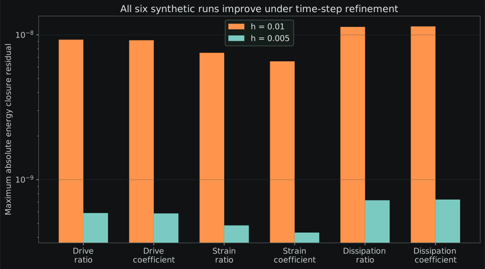
No manufactured forcing is present in these train/rest/probe runs. R = E − Wdrive + Q − Wparam; each row reports max |R| across the trajectory in normalized energy units. Phase boundaries are aligned to both grids.
| Writing / damping | max |R|, h=.01 | max |R|, h=.005 | Residual ratio | |Δ probe RMS| |
|---|---|---|---|---|
| drive / ratio | 9.2635859e-09 | 5.8826705e-10 | 15.747 | 2.7998983e-07 |
| drive / coefficient | 9.1815339e-09 | 5.8483529e-10 | 15.699 | 3.0310902e-07 |
| strain / ratio | 7.5161997e-09 | 4.8320392e-10 | 15.555 | 1.9305168e-07 |
| strain / coefficient | 6.5673271e-09 | 4.3103565e-10 | 15.236 | 2.4016719e-07 |
| dissipation / ratio | 1.1350696e-08 | 7.2065667e-10 | 15.750 | 1.8219585e-07 |
| dissipation / coefficient | 1.1446152e-08 | 7.2899035e-10 | 15.701 | 2.5472104e-07 |
Python–JavaScript cross-check: original model only
| h | Quantity | Python | Browser solver in Node | Absolute difference |
|---|---|---|---|---|
| 0.01 | probe_rms | 0.873555668884 | 0.873555668884 | 3.331e-16 |
| 0.01 | max_energy_residual | 9.26358589837e-09 | 9.26358723063e-09 | 1.332e-15 |
| 0.01 | q | -0.898949012897 | -0.898949012897 | 1.110e-15 |
| 0.01 | p | -1.30085284006 | -1.30085284006 | 8.882e-16 |
| 0.01 | m | 0.206623596516 | 0.206623596516 | 2.776e-17 |
| 0.005 | probe_rms | 0.873555388894 | 0.873555388894 | 0.000e+00 |
| 0.005 | max_energy_residual | 5.88267046187e-10 | 5.88272541791e-10 | 5.496e-15 |
| 0.005 | q | -0.898949014291 | -0.898949014291 | 0.000e+00 |
| 0.005 | p | -1.30085283928 | -1.30085283928 | 0.000e+00 |
| 0.005 | m | 0.206623596516 | 0.206623596516 | 0.000e+00 |
The browser solver was executed in Node; this does not test browser interaction or Google Analytics. Both implementations share equations and inputs and were run within this project. Full precision output · Reproduction script
Project controls at a glance
| Control | Computed result | Scope |
|---|---|---|
| P01 end correction | Δ = −0.079879 mm; conditional 95% profile interval [−0.411662, 0.251949] mm | Synthetic 12-row likelihood and uncertainty |
| P03 positive break | Held-out MSE difference 0.036199583; bootstrap interval [0.016451374, 0.057375485] | Synthetic data generated with a break |
| P03 single-power-law null | Difference 0.000127982; interval [−0.000239906, 0.000471207] | The interval includes zero; 87/200 null simulations favor the hinge on raw held-out MSE, without a decision threshold. |
Three evidence gates, without a rating
| Gate | Required evidence | Current position |
|---|---|---|
| 1. Inspectable claims | Source roles, explicit equations, baseline, uncertainty and a failure criterion for every operational claim. | Documentation revised; independent scientific audit remains open. |
| 2. Independent reproduction | A reviewer outside this authoring process reproduces the named release and reports environment, discrepancies and conflicts. | No independent human reproduction received. |
| 3. Empirical discrimination | A frozen analysis predicts genuinely untouched observations and is compared with adequate conventional rivals. | No completed decisive experiment or validated measured fit. |
The private AI-assisted desk review prompted this work. Its numerical rubric is not used as scientific evidence. The public response record explains each accepted correction and remaining disagreement without publishing private correspondence. Independent review packet and publication status
Downloads
Complete research release · SHA-256 catalogue · Model results · Acoustic results